Introduction/Background
Winning is everything to Formula 1 teams as victory brings an increase in brand value, revenue and team pride. Optimizing parameters such as race strategies, car setups, and driver selection is crucial to come out on top. Formula 1 teams collect large quantities of data such as weather data, car telemetry data, or rival radio messages. Portions of this data are publicly available. One group used brake and telemetry data from previous races and associated the data to specific drivers using neural networks and random decision trees [1]. A researcher at Amazon evaluated different models to predict drivers’ qualifying position based on their practice performance during that race weekend [2]. Some groups used techniques such as deep learning and support vector machines to predict race positions and the overall winner [3,4].
Dataset Description/Link
Ergast is an API for querying Formula 1 Race records. The database contains race information such as constructors, drivers, lap times, pit stops, qualifying, and results. Fast-F1 and OpenF1 are APIs for accessing live timing/telemetry data. These APIs provide access to individual race car telemetry data, such as speed, RPM, gear, and throttle.
Problem Definition
Qualifying is a critical part of a Formula 1 Race. It determines starting positions for each driver. Each driver’s goal is to extract the fastest lap out of their cars during qualifying. Predicting the driver’s qualifying time can provide a driver specific benchmark for each session, helping teams evaluate performance, tailor strategy, and increase the excitement of fans, gamblers, and broadcasters.
As the car, track, weather, and tires can change between seasons and sessions we propose developing a model that utilizes performance data from practice sessions and the active qualifying session (drivers have multiple attempts in qualifying) to predict the qualifying performance of a driver.
Methods and Analysis
Data Filtering and Cleaning
For the initial data preprocessing and cleaning, we elected to choose 4 features, namely the fastest lap time amongst all three practice laps, and speed tests at multiple speed traps across all practice laps. These features are a preliminary insight into how different drivers fare across practice laps, and would translate well to the actual race lap placement.

Additionally, to have clean and actionable data, we filter data based on if the weather was rainy, in which case the distribution of time and kind of driving changes. For an initial look we wished to evaluate the naïve clustering techniques on an easier task, and hence we remove any events that have rainy weather. Red flags signify accidents or some other sort of hindrance to the race, and usually signal emergency. Since these events are outliers and anomalies, we filter out those as well. We also only took data from 2022 onwards as the new F1 regulations started that year.
As part of data exploration, we performed PCA on the data, where we see, as expected, a heavy reliance on the track for the qualifying lap time, and therefore whilst clustering, we adopted the approach of normalizing the dataset by accounting for different tracks.

The difference between the figure above and below is that we normalized the data by the track the time was completed on. As you can see this causes a drastic change as before the normalization the PCA algorithm was just clustering by track and providing no new substantial insight into the data.

A visual representation of our data preprocessing can be seen under the clustering visualizations section.
Data Changes made for 1D CNN
Because neural networks require much more data and we wanted to evaluate temporal (time-series) data, we decided to make the following changes to our preprocessing workflow. We increased our sample size by now taking data from 2013 onwards. We investigated using time series telemetry data reported by sensors on board every car. This data includes the speed of the car, the engine RPM, the gear the car is in, the percentage of the throttle used, and the position of the car along the track. We decided to normalize this data with respect to the relative distance along the track for each car. This ensures that we have the same number of data points in each time series, regardless of actual time spent driving the lap, and accounts for varying track lengths across different sessions. The below figures show two examples of this time series data for Max Verstappen and Lewis Hamilton during the first practice session of the Monaco 2022 Grand Prix. We can see that although the initial data is reported as time series data, we include time itself as a feature in this dataset.
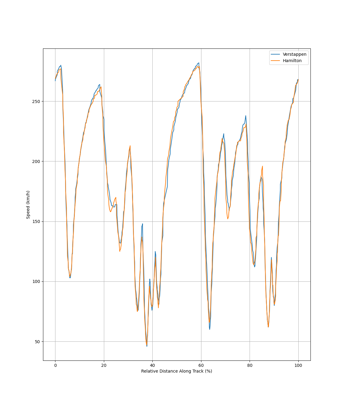
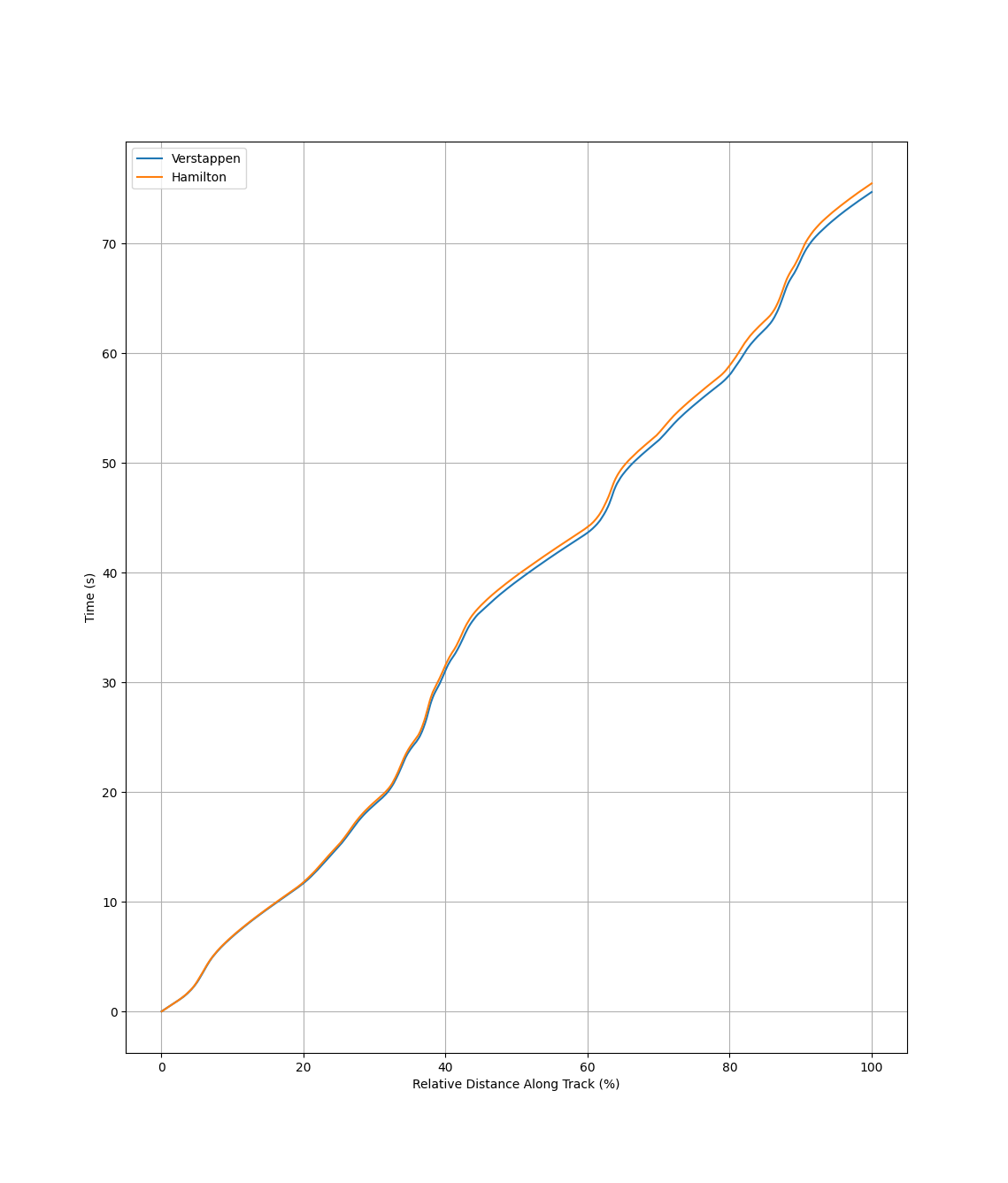
For each driver in each grand prix, data from on-board telemetry is condensed into 15 features: time, speed, rpm, car gear, and throttle from the fastest lap for each of the three practice sessions. Each feature is further condensed into 100 individual data points, representing the average measurement for 1/100th of the distance traveled during that lap. A visual representation of our data preprocessing can be seen under the 1D CNN visualizations section.
Data Augmentation
The raw telemetry data used is not perfect, and there are several instances of unavailable data in the dataset. Data that is represented as NaN in the dataset was filled in using a backfill method, where the next available data point is substituted into any NaN values.
For the purposes of the 1D Convolutional Neural Network, we found that the existing data samples were insufficient to train a model with good confidence. While we worked on generating more data, we utilized methods of data augmentation to supplement our data and oversample on the given data to produce actionable model learning. We utilized the addition of random gaussian noise to the existing time-series data of different features to have newer augmented data that the model can train on.
Data Changes made for Random Forest
We decided to change our data filtering method from the intital EDA from clustering. We went back one year (2021) to get more data, and we also allowed incomplete race weekends (1-3 practice sessions) to increase our sample size. However, for incomplete race weekends, at least one practice session and qualifying must not have a red flag. We also extracted more features that we believed could improve the performance of the random forest model: practice ranking, driver name, and team name. We encoded the driver name and team name to make our data compatible with scikit learn’s random forest model. A visual representation of our data preprocessing can be seen under the random forest visualizations section.
ML Methods and Analysis
Clustering (Unsupervised Learning):
Due to the complex relations that we might observe, we identify DBScan and Gaussian Mixture Models as two potential clustering models due to their soft clustering. Based on the performance we might also consider popular models such as K-Means(hard clustering).
DBScan:
Due to its inherent nature of inferring clusters based on proximity and neighbor nodes, we used DBScan to cluster and classify the drivers based on their features.
Gaussian Mixture Models :
Gaussian Mixture models were chosen due to their diverse nature of being able to model the dataset as a mixture of Gaussians, which can translate well with our numeric data features.
Random Forest (Supervised Learning):
We thought a random forest would be useful as its bagging has an inherent benefit for our multi-class classification since we are trying to predict the rankings for twenty different drivers. The random forest’s first choice is also its most impactful, so we can see which features from our dataset give the model the most information. This combined with its robustness for outliers, which can be common due to all of the uncertainty during the races, makes the Random Forest a good match for what we are triyng to accomplish.
1D Convolutional Neural Network (Supervised Learning):
We chose to use a CNN to try and capture the intricacies of the time series data in each lap. With time series we are splitting each lap into 100 time intervals that each have their own specific value for each of our features. That means for each lap we have d*100 parameters that we can utilize.
The parameters we chose to utilize in the CNN are
| Feature | Description |
|---|---|
| Time | Total seconds elapsed |
| Speed | Speed of the car at that instance |
| RPM | Engine speed or how fast the engine’s crankshaft is rotating. |
| nGear | Gear the F1 car is in at each timestamp |
| Throttle | Degree to which the accelerator is pressed |
| Relative Distance | Relative distance of the track covered |

We utilize a 1D ConvNet with 26,333 parameters, with convolutions followed by a Rectified Linear Unit to bring non-linearity, and a maxpool layer for aggregation. The features are flattened and passed through a Fully Connected layer to yield the final qualifying time based on all metrics of the first three practice laps.
Results + Discussion:
Visualizations:
Clustering Algorithms (GMM & DBSCAN)

1D CNN

| Hyperparameter | Value |
|---|---|
| Learning Rate | 0.0001 |
| Optimizer | Adam |
| Batch Size | 150 |
| Num Epochs | 1200 |
Random Forest

The performance of random forest can be improved by tuning the hyperparameters, such as number of trees in the forest, maximum depth, minimum number of samples required to split, etc. The number of trees in the forest is one of the most important parameter associated with random forest. The following graph demonstrated that as the number of tree increases, the root mean squared error of the regression decreases. However, after certain threshold, the improvement in accuracy becomes negligible.

One of the advantage of using random forest is its ability to differentiate the importance of features. Random forest can measure the importance of features by maximizing the information gain. The combined decisions of the forest can reveal which features are important, which helps user eliminate less important features, reducing the dimensionality of the train data, and improve the overall performance. The relative importance of the features are ranked in the following graph. The result indicates that the total lap time and ranking of each practice runs are the most important for predicting the qualifying time.

We used cross validation and grid search for the hyperparameter tuning process. Through the tuning process, we were able to find the best parameters for our random forest implementation.
| Hyperparameter | Value |
|---|---|
| n_estimators | 200 |
| max_depth | 80 |
| max_features | sqrt(D) |
| min_samples_leaf | 1 |
| min_samples_split | 10 |
The graph below visualize an sample tree in the random forest using the above parameters.

Quantitative Metrics
We see that, in general, simple unsupervised clustering algorithms do not perform well when we try to capture the relationship of finishing position inherently. This is due to multiple reasons. Firstly it could be that multiple different drivers adapt similar strategies even though they might not finish in the same places.
Due to the nature of the different strategies adopted to test the track during the practice laps, the simple translation of finish times in practice laps does not translate to actual race finishing position. Hence why, in our next steps we aim to explore more diverse and varied features in order to capture inherent mechanics behind the practice laps that can be translated towards final position predictions.
DBScan
| Hyperparameters | Value |
|---|---|
| eps | 0.7 |
| Clustering Results | Value |
|---|---|
| # of clusters | 10 |
| # of noise points | 31 |
| Metrics | Value |
|---|---|
| Homogeneity | 0.301 |
| Completeness | 0.467 |
| V-measure | 0.366 |
| Adj. Rand Index | -0.019 |
| Adj. Mutual Info | -0.057 |
| Silhouette Coeff. | 0.027 |
GMM
| Hyperparameters | Value |
|---|---|
| # of clusters | 20 |
| Metrics | Value |
|---|---|
| Homogeneity | 0.575 |
| Completeness | 0.598 |
| V-measure | 0.586 |
| Adj. Rand Index | 0.021 |
| Adj. Mutual Info | 0.036 |
| Silhouette Coeff. | 0.206 |
1D CNN
| Model Parameters | MSE | MAE | RMSE | R2 |
|---|---|---|---|---|
| 11k parameters | 2.5 | 1.32 | 1.58 | 2.9 |
| 5k parameters | 6.7 | 3.12 | 2.59 | 7.8 |
| 70k parameters | 2.2 | 1.09 | 1.48 | 3.1 |
| 26k parameters | 0.5690 | 0.5835 | 0.45 | 0.76 |
Random Forest
| Model | Explained Variance | MSE | MAE | RMSE | R2 |
|---|---|---|---|---|---|
| Random Forest | 0.7361 | 0.2258 | 0.3744 | 0.4752 | 0.7270 |
Analysis of models
DBScan
The DBScan algorithm scored under .5 for homogeniety and completeness metrics. Due to not being able to assign the number of clusters, there is a huge disagreement between true labels and predicted labels. DBScan fails to properly classify the drivers’ finishing position.
Gaussian Mixture Models
With GMM both stats were right around .6 for both homogeniety and completeness. This metric helped us measure our improvements as after we had normalized our data based on the track the time was from, the homogeneity and completeness values increased by .1 for our GMM model after this normalization.
1D Convolutional Neural Network
We utilized different variants of a 1D Convolutional Neural Network with time dependant features. We extracted the time series data of a car’s Speed, Brake, RPM, Throttle and the Relative Distance completed in the lap. We chose these features, as they all represent the state of the car throughout the race rather than an average, and the Relative Distance feature is responsible for grounding the speed with respect to different race tracks and different conditions. We use these features convoluted through the 1D convolution to predict the final qualifying time.
We observe that the data required for the convolutional network was far more than what was required for the other methods. Along with processing data from the past 10 years, we further imputed the data using data augmentation methods specified above to create new augmented samples. With the help of these augmentations, the model was able to learn exceedingly well, generalizing to the dataset and possible noise through the augmentations.
Random Forest
To improve the performance of random forest model, we added categorical data, driver and team information, to the training data. To find the best hyperparameters for the random forest model, we employed K Fold cross validation and grid search techniques. The hyperparameters that were most successful for our data is using bootstrap, 200 trees, sqrt(D) features, maximum tree depth of 80, minimum number of samples to split at 10, and minimum number of samples at a leaf node at 1.
Using the existing data without further data augmentation, the model is already capable of predicting qualifying time at a similar performance to other methods. This indicates that random forest can be an effective methods for this regression problem. Another advantage of the random forest is the extremely low time and resource requirement for training the model while yielding acceptable results.
Comparison of Models
| Model | Homogeneity | Completeness | V-measure | Adj. Rand Index | Adj. Mutual Info | Silhouette Coeff. |
|---|---|---|---|---|---|---|
| GMM | 0.575 | 0.598 | 0.586 | 0.021 | 0.036 | 0.206 |
| DBSCAN | 0.301 | 0.467 | 0.366 | -0.019 | -0.057 | 0.027 |
Our GMM and DBSCAN both did not perform great, but the GMM performed much better relatively to DBSCAN in all the metrics shown. Our GMM model was able to form more pure, complete, and distinct clusters over DBSCAN. Also, we were not able to find a hyperparameter value that yielded 20 clusters with DBSCAN, which from that alone, cannot help us in our goal of predicting qualifying order. Ultimately, clustering is not a great method for predicting qualifying order.
| Model | Explained Variance | MSE | MAE | RMSE | R2 |
|---|---|---|---|---|---|
| Random Forest | 0.7361 | 0.2258 | 0.3744 | 0.4752 | 0.7270 |
| 1D CNN | N/A | 0.5690 | 0.5835 | 0.45 | 0.76 |
When comparing our supervised learning methods, the performances are really close. The mean squared error and mean absolute error easily goes to the Random Forest model, but the 1D CNN performs better in the root mean squared error and R-squared metrics. The RMSE value indicates that the 1D CNN predictions are just barely closer than the Random Forest. The R-squared value also shows that the 1D-CNN is able to capture a greater proportion of the variance in the qualifying order. Thus, while very close to each other, the 1D CNN performed better than the Random Forest.
Our 1 dimensional CNN performed the best, with random forest coming in a very close second. Our gaussian mixture model and DBSCAN performed much worse than our supervised methods, but the performance of the gaussian mixture model was much better than DBSCAN.
Next Steps:
Feature Engineering:
We can consider expanding our important features by conducting feature importance analysis to see what other information our data has that can help predict qualifying race times. We can explore other domain-specific features such as track characteristics (like track temperature), car specifications, or other features that could improve predictions by helping capture more linear, non-linear, or temporal dependencies hidden in our data.
Re-evaluation of Clustering:
We can continue to incorporate additional domain knowledge/constraints to help our clustering. We’ve already seen benefits from normalizing databases on track, so other variables such as racing strategies, or driver teams might also yield similar results. We could look for certain features that we believe would cluster better and apply feature engineering to allow DBSCAN or a GMM to perform better.
Supervised Learning:
We can compare and contrast the results gained when we implement Gradient boosted regression and a simple Neural Net. We can experiment with different structures and hyperparameters for the neural net to try and increase it’s potency.
Evaluation Metrics:
We can continuously monitor model performance using a variety of evaluation metrics beyond Mean Squared Error and R2 , such as MAPE, precision, recall, or F1 score to gain a more comprehensive understanding of model performance.
Data Preprocessing:
With our initial dataset we eliminated outlying data such as rainy weather or red flag event. If we find a way to increase our model’s accuracy we could possibly try and use the rain affected times to allow our model to try and predict qualifying times based on weather, as not every race will have perfect conditions.
Future Experimentation:
We can implement a systematic approach to experimentation by maintaining clear documentation of experimental setups, results, and insights gained from each iteration.
References
[1] J. von Schleinitz, L. Wörle, M. Graf, A. Schröder and W. Trutschnig, “Analysis of Race Car Drivers’ Pedal Interactions by means of Supervised Learning,” 2019 IEEE Intelligent Transportation Systems Conference (ITSC), Auckland, New Zealand, 2019, pp. 4152-4157, doi: 10.1109/ITSC.2019.8917120.
[2] Yang, Guang. “Predicting Qualification Ranking Based on Practice Session Performance for Formula 1 Grand Prix.” AWS Machine Learning Blog, 13 Nov. 2020, aws.amazon.com/blogs/machine-learning/predicting-qualification-ranking-based-on-practice-session-performance-for-formula-1-grand-prix/.
[3] B. Peng, J. Li, S. Akkas, T. Araki, O. Yoshiyuki and J. Qiu, “Rank Position Forecasting in Car Racing,” 2021 IEEE International Parallel and Distributed Processing Symposium (IPDPS), Portland, OR, USA, 2021, pp. 724-733, doi: 10.1109/IPDPS49936.2021.00082.
[4] P. Shelke, A. Pande, S. Kale, Y. Paralikar and A. Kulkarni, “F1 Race Winner Predictor,” 2023 7th International Conference On Computing, Communication, Control And Automation (ICCUBEA), Pune, India, 2023, pp. 1-4, doi: 10.1109/ICCUBEA58933.2023.10392224.
Gantt Chart

Contributions
| Name | Proposal Contributions |
|---|---|
| Wesley Ford | Problem Descrption & Motivation, Potential Results & Discussion, Video Presentation |
| Nathan Chung | Introduction, Problem Description & Motivation, Video Presentation |
| Ryan Bard | Introduction, Methods, Results & Discussion, GitHub repository management |
| Yu Hang He | Introduction, Dataset, References |
| Aryan Vats | Methods, Potential Results & Discussion |
| Name | Midterm Contributions |
|---|---|
| Wesley Ford | Data Cleaning and Preprocessing |
| Nathan Chung | Data Cleaning, Visualizations, PCA |
| Ryan Bard | Next Steps, Analysis, Visualizations, Report Writeup |
| Yu Hang He | Implementation of GMM and DBScan |
| Aryan Vats | Methods, Visualizations, Analysis, Report Writeup |
| Name | Final Contributions |
|---|---|
| Wesley Ford | Data Cleaning and Preprocessing for ConvNet, Visualizations, Final Report, Final Video |
| Nathan Chung | Data Cleaning and Preprocessing for RandomForest, Visualizations, Final Report, Final Video |
| Ryan Bard | Visualizations, Report Writeup, Final Video, experimentation of ConvNet |
| Yu Hang He | Implementation of RandomForest and experimentation, Visualizations, Final Report |
| Aryan Vats | Implementation of ConvNet and experimentation, Final Report, Final Video |